8 ways to clean data in excel (part 1)

You cannot always have control over the format and type of data you import from a database, a text file or a web page. Before we can analyse the data, we often need to do a good cleaning.
Fortunately, Excel has many features to get the data in the exact format we want. Sometimes the task is simple and sometimes it requires more steps. In the following we will take a look at 8 ways (4 in this first part) to clean data in Excel.
1. Spelling check
We can use a spell checker not only to find misspellings, but also to look up values that are not used consistently, such as product or company names, by adding these values to a custom dictionary.
- Use the following instructions to check spelling and grammar in Excel 2007.
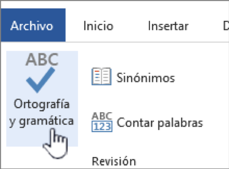
Open the spelling and grammar checker. In the Checkin the review group, click on Spelling. If the programme finds spelling errors, the first misspelled word or grammatical error is highlighted. The options you see vary slightly depending on which version you are using and whether the error is a spelling or grammatical mistake.
- Use the following instructions to check spelling and grammar in Excel 2010 and later for Windows.
To start the spelling and grammar check on the file press F7 or follow these steps:
1- Click on the tab Check from the ribbon.
2- Click on Spelling or Spelling and grammar.
3- If the programme finds spelling mistakes, a dialogue box will appear with the first misspelled word found by the spellchecker.
4- When you have decided how to resolve the spelling mistake (omit, change or add to the programme's dictionary), the checker will move on to the next incorrect word.
- Use the following instructions to spell check in Excel for Mac
Remember that you can check spelling, but you cannot check grammar. To check all spelling at once:
- In the tab Checkclick on Spelling.
Note: The dialogue box spelling will not open if no spelling errors are detected or if the word you are trying to add already exists in the dictionary.
Do one of the following:
| For | Perform this procedure |
| Change the word | At SuggestionsClick on the word you want to use and then click on Change. |
| Change all occurrences of this word in the document | At SuggestionsClick on the word you want to use, and then click on Change everything. |
| Omit this word and move on to the next misspelled word. | Click on omit once. |
| Omit each occurrence of this word in the document and move on to the next misspelled word. | Click on Omit everything. |
2. Remove duplicate rows
Duplicate rows are a common problem when importing data. It is a good idea to first filter by unique values to confirm that the results are what you want, before removing duplicate values.
Filter out single values y remove duplicate values are two similar tasks, since the objective is to present a list of unique values. However, there is a critical difference: when filtering unique values, duplicate values are only temporarily hidden. However, when removing duplicate values, duplicate values are permanently removed.
Check before removing duplicates: Before removing duplicate values, it is a good idea to try filtering for unique values, or conditional formatting, to confirm that you get the results you expect.
- Filter out single values
Follow these steps:
1- Select the range of cells or make sure that the active cell is in a table.

2- Click on > advanced data (in the group sort & filter).
3- In the pop-up message box advanced filterIf you do not do so, do one of the following:
To filter the range of cells or the table instead:
- Click on filter the list, in context.
To copy the filter results to another location:
- Click Copy to another location.
- In the table Copy toenter a cell reference.
- Alternatively, click collapse from dialogue to temporarily hide the pop-up window, select a cell in the spreadsheet, and then click on expand.
- Check only unique records and then click on Accept.
The unique values of the range will be copied to the new location.
- Remove duplicate values
When removing duplicate values, the only effect applies to values in the range of cells or table. Other values outside the range of cells or table do not change or move. When duplicates are removed, the first occurrence of the value in the list is retained, but other identical values are removed.
Because it permanently deletes data, it is a good idea to copy the original range of cells or table to another spreadsheet or workbook before removing duplicate values.
Follow these steps:
1- Select the range of cells or make sure that the active cell is in a table.
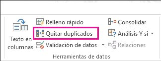
2- In the tab dataclick on remove duplicates (in the tools group of data).
3- Carry out one or more of the following procedures:
- At Columnsselect one or more columns.
- To quickly select all the columns, click on Select all.
- To quickly delete all the columns, click on Unselect. If the range of cells or table contains many columns and you only want to select some of them, you will find it easier to click on Unselect and then in Columnsselect these columns.
Note: The data will be removed from all columns, even if you do not select all columns in this step. For example, if you select Column1 and Column2, but not Column3, the "key" used to search for duplicates is the column value Column1 & Column2. If a duplicate is found in those columns, the entire row will be removed, including other columns in the table or range.
4- Click on Accept and a message will appear to indicate how many duplicate values have been removed or how many unique values are retained. Click on Accept to close the message.
5- If you do so, click unDo (or press Ctrl + Z on your keyboard).
3. Find and replace text
You may want to remove a common initial string, such as a tag followed by a colon and a space, or a suffix, such as a secondary phrase at the end of the string that is obsolete or unnecessary. To do this, you can search for instances of such text, and then replace it with no text or other text.
Use the features Search and replace in Excel to search for items in your workbook, such as a particular number or text string.
1- In the tab Home in the group Editionclick on Search and select.

2- Follow one of these procedures:
- To search for text or numbers, click on Search.
- To search for and replace text or numbers, click on Replace.
3- In the table SearchIf you want to search, type in the text or numbers you want to search for, or click on the arrow in the box. Search and then click on a recent search in the list.
You can use wildcard characters, such as an asterisk (*) or a question mark (?), in your search criteria:
- Use the asterisk to search for any character string. For example, s*l will return both "salt" and "signal".
- Use the question mark to search for a single character. For example, it will return "salt" and "sun".
SuggestionYou can search for asterisks, question marks and tilde characters (~) in spreadsheet data by prefixing a tilde character in the Search box. For example, to search for data containing "?", you would type ~? as the search criteria.
4- Click on Options to further define the search if necessary:
- To search for data in a spreadsheet or an entire workbook, in the Within box, select Sheet or Book.
- To search for data in rows or columns, in the Find box, click on By rows or By columns.
- To search for data with specific details, in the Search within box, click on Formulas, Values or Comments.
Note: Formulas, values, notes and comments are only available on the Find tab; only formulas are available on the Replace tab.
- To search for case-sensitive data, select the checkbox Matching upper and lower case letters.
- To search for cells that contain only the characters you typed in the Find box, select the Match contents of the whole cell.
5- To replace text or numbers, type in the new text or number in the box Replace with (or leave the box blank so as not to replace the characters with anything), and then click on Search o Search all.
Note: If the table Replace with is not available, click on the tab Replace.
If you wish, you can cancel an ongoing search by pressing ESC.
6- To replace the highlighted match or all the matches found, click on Replace o Replace all.
4. Changing the capitalisation of text
Sometimes text is a mixture, especially when case is concerned. By using one or more of the three case functions, you can convert text to lower case, such as email addresses, upper case, such as codes, or upper or lower case, such as first or last names.
You can use the functions MAYUSC, MINUSC o NOMPROPIO to automatically convert existing text from lowercase to uppercase, from uppercase to lowercase, or to proper name format. Functions are simply built-in formulas that are designed to perform specific tasks (in this case, switching between upper and lower case).
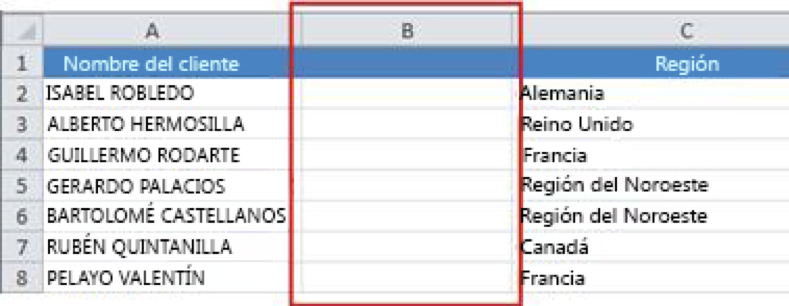
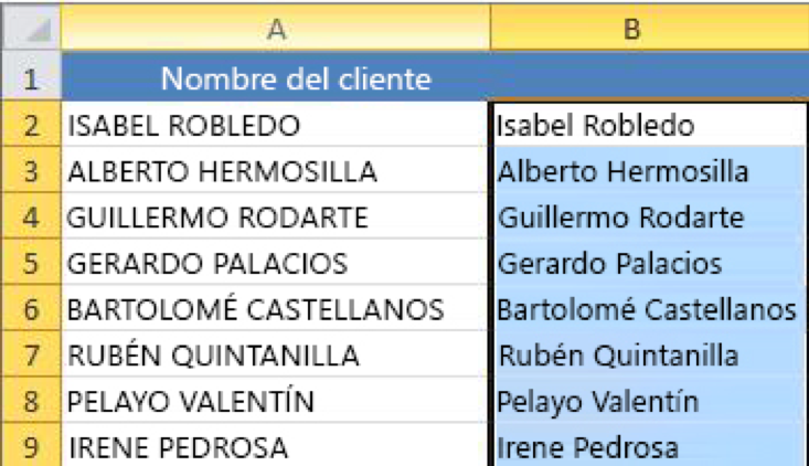
In the following example, the function NOMPROPIO is used to convert the capitalised names in column A to proper names, so that only the first letter of each name is capitalised.
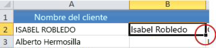
1- First, insert a temporary column next to the column containing the text you want to convert. In this case, we have added a new column (B) to the right of Client's name.
In cell B2, type =PROPIOUSNAME(A2), and press Enter.
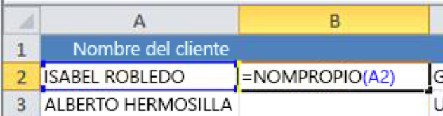
This formula converts the name in cell A2 to a proper name. To convert the text to lower case, enter =MINUSC(A2). Use =MAYUSC(A2) when you want to convert text to uppercase by replacing A2 with the appropriate cell reference.
2- Now, fill down the formula in the new column. The quickest way to do this is to select cell B2 and double-click on the small square in the bottom right-hand corner of the cell.
Suggestion: If your data is in an Excel table, a calculated column is automatically created with the values filled in when you enter the formula.
3- At this point, the values of the new column (B) must be selected. Click on Ctrl+C to copy them to the clipboard.
Right-click on cell A2, click on the cell, click on Paste and then click on Values. This step allows you to paste only the names and not the underlying formulas, which you do not need to keep.
4- You can delete column (B), as it is no longer necessary.
Well, so much for these first 4 ways to clean up data in Excel. In the next post, we will look at the 4 remaining ways we have yet to illustrateWe hope you find this information useful!