8 ways to clean data in excel (part 2)

In the previous post, 8 ways to clean data in excel (part 1)In the first part, we looked at the first 4 ways to clean up data in excel: spell checking, removing duplicate rows, finding and replacing text, and finally, changing the capitalisation of text. In this second part we will look at the last 4 ways we have yet to see. Take note!
5. Removing spaces and unprintable characters from the text
Sometimes text values contain embedded space characters in the first part, at the end or in several places.
Often, these characters can produce unexpected results when sorting, filtering or searching. For example, in the external data source, users may make typographical errors by inadvertently adding extra space characters or importing text data from external sources that may contain non-printable characters that are embedded in the text. Because these characters are not easily observed, it can be difficult to understand the unexpected results. To remove these unwanted characters, you can use a combination of the functions SPACES y REPLACE.
A) Function SPACES
Removes spaces in the text, except for the normal space between words. Use SPACES in text from other applications that may contain irregular spacing.
Syntax
SPACES (text)
The syntax of the function SPACES has the following arguments:
- Mandatory Text. This is the text from which you want to remove spaces.
B) Nuncio REPLACE
Replaces original_text with new_text within a text string. Use REPLACE to replace specific text in a text string.
Syntax
REPLACE (text, original_text, new_text, [occurrence_number])
The syntax of the function REPLACE has the following arguments:
- Mandatory Text. This is the text or reference to a cell containing the text in which you want to replace characters.
- Original_text Mandatory. This is the text you wish to replace.
- New_text Mandatory. This is the text you want to replace the original_text with.
- Occurrence_number Optional. Specifies the instance of original_text to replace with new_text. If you specify the occurrence_number argument, only that instance of original_text is replaced. Otherwise, all instances of original_text in text will be replaced by new_text.
6. Correct date values
Because there are different date formats and these formats can be confused with numbered element codes or other strings containing slashes or hyphens, it is often necessary to convert and reformat date values.
- Convert dates stored as text to dates
Sometimes dates can be formatted as text and stored as text in cells. For example, you may have typed a date in a cell with text formatting, or the data may have been imported or pasted from an external data source as text.
Dates with text formatting are aligned in a cell to the left (instead of to the right). When the error checking is enabled, text dates with two-digit years can also be marked with an error indicator: .
Since error checking in Excel can detect text-formatted dates with two-digit years, you can use the automatic correction options to convert them into date-formatted dates. You can use the function DATENUMBER to convert most types of dates from text to dates.
- Function DATENUMBER:
To convert a text date in a cell to a serial number, use the function DATENUMBER. Next, copy the formula, select the cells containing the text dates and use Special gluing to apply a date format to them.
Follow these steps:
- Select a blank cell and check that the number formatting is General.
- In the blank cell:
- Write = DATENUMBER (
- Click on the cell containing the text-formatted date you want to convert.
- Enter )
- Press enter and the function DATENUMBER returns the serial number of the date represented by the text date.
What is an Excel serial number?
Excel stores dates as sequential serial numbers so that they can be used in calculations. By default, 1 January 1900 is serial number 1 and 1 January 2008, which is serial number 39448 because it is 39,448 days after 1 January 1900. To copy the conversion formula into a range of contiguous cells, select the cell containing the entered formula, then drag the fill handle into a range of empty cells that matches in size the range of cells containing the text dates.
- After dragging the fill handle, you should have a range of cells with serial numbers that corresponds to the range of cells containing the text dates.
- Select the cell or range of cells that contains the serial numbers, then right-click and select copy.
- Select the cell or range of cells containing the text dates and right-click and select Special gluing.
- In the dialogue box Special gluingin Paste, select Values and click on Accept.
- In the tab HomeClick on the selector in the pop-up window next to number.
- In the table Categoryclick on Date and, in the list TypeClick on the date format of your choice.
- To remove the serial numbers after all dates have been successfully converted, select the cells containing them, then press the DELETE.
7. Merge and split columns
A common task after importing data from an external data source is to combine two or more columns into one, or to split one column into two or more columns. For example, you could split a column containing a full name into a first and last name. Or you could split a column containing an address field into separate street, city, region and postcode columns. The reverse can also be true. You might want to combine a first and last name column into a full name column or combine separate address columns into a single column.
Merge data from different cells, e.g. first and last names.
- Combine data with the symbol (&)
- Select the cell in which you want to put the merged data.
- Type = and then select the first cell you want to merge.
- Write & and enclose a blank space in quotation marks.
- Select the next cell you wish to merge and press Enter. An example formula could be =A2&" "&B2.
or by using the formula CONCATENAR
- Combining data with the CONCAT function
- Select the cell in which you want to put the merged data.
- Write =CONCAT(
- Select the cells you want to merge first.
Use semicolons to separate cells you want to merge and use inverted commas to add spaces, commas or additional text. - Close the formula with a parenthesis and press Enter.
Split text into different columns with the Convert Text into Columns Wizard
You can place the text in one or more cells and split it into several cells with the Assistant to convert text into columns.
- Select the cell or column containing the text you want to split.
- Select Data > Text in Columns.
- In the Convert Text to Columns Wizard, select Delimited > Next.
- Select the Boundary markers for their data. For example, Coma y Space. You can see a preview of the data in the window Data preview.
- Select Next.
- Select the Column data format or use the Excel hint.
- Select the Destinationwhich is where you want the split data to appear in the spreadsheet.
- Select End.
8. Transform and rearrange columns and rows
Most of the analysis and formatting features in Office Excel assume that the data exists in a single flat two-dimensional table. Sometimes, you may want to make rows into columns and columns into rows. Other times, the data is not even structured in a tabular format and you need to be able to transform it from a non-tabular to a tabular format.
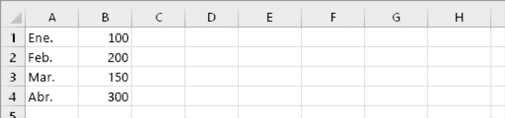
Sometimes you will need to change or rotate cells. To do this, you can copy, paste special and use transposition option. But doing so creates duplicate data. To avoid this, you can write a formula instead of using the TRANSPONER function. For example, in the following picture, the formula =TRANSPOSE(A1:B4) takes cells A1 to B4 and arranges them horizontally.
The key to making TRANSPONER work: Be sure to press CTRL+SHIFT+ENTER after typing the formula. If you have never typed this type of formula before, the following steps will guide you through the process.
Step 1: Select blank cells
First select a number of blank cells. But make sure you select the same number of cells as in the original set of cells, but in the opposite direction. For example, here are 8 cells arranged vertically:
Therefore, we have to select eight horizontal cells, like this:
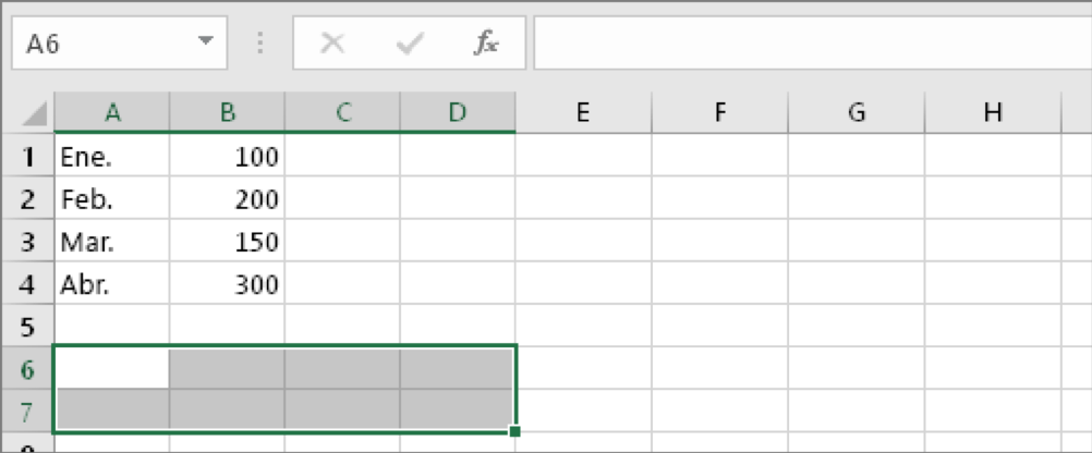
This is where the new cells will end up after transposition.
Step 2: Type =TRANSPONER(
With the same blank cells selected, type: =TRANSPONER(
Excel will look similar to the following:
Notice that all eight cells are still selected even though we have started typing a formula.
Step 3: Write the range of the original cells.
Now, type in the range of cells you want to transpose. In this example, we want to transpose cells A1 to B4. The formula for this example would then be: =TRANSPOSE(A1:B4); but do not press ENTER yet. Just stop writing and go to the next step.
Excel will look similar to the following:
Step 4: To finish, press CTRL+SHIFT+ENTER.
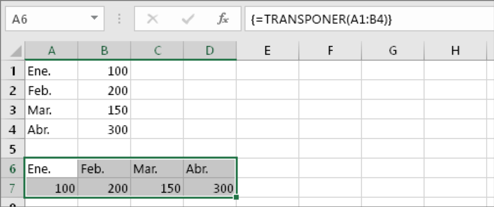
Now press CTRL+SHIFT+ENTER. Why? Because the TRANSPONER function is only used in matrix formulae and this is the way to finish an array formula. In short, an array formula is a formula that applies to more than one cell. As you selected more than one cell in step 1, the formula will be applied to more than one cell. This is the result after pressing CTRL+SHIFT + ENTER:
And here are the last 4 ways to clean data in excel. Remember that this post is divided in 2 parts and that we saw the first 4 forms in the previous post. If you have missed it, we recommend you take a look at it.